Connect with us

The Conversation

What’s that microplastic? Advances in machine learning are making identifying plastics in the environment more reliable

Published

on

theconversation.com – Ambuj Tewari, Professor of Statistics, University of Michigan – 2025-03-06 07:35:00

Microplastics are tiny bits of plastic that show up in the environment.
Svetlozar Hristov/iStock via Getty Images Plus

Ambuj Tewari, University of Michigan

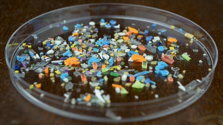
Microplastics – the tiny particles of plastic shed when litter breaks down – are everywhere, from the deep sea to Mount Everest, and many researchers worry that they could harm human health.

I am a machine learning researcher. With a team of scientists, I have developed a tool to make identification of microplastics using their unique chemical fingerprint more reliable. We hope that this work will help us learn about the types of microplastics floating through the air in our study area, Michigan.

Microplastics – a global problem

The term plastic refers to a wide variety of artificially created polymers. Polyethylene, or PET, is used for making bottles; polypropylene, or PP, is used in food containers; and polyvinyl chloride, or PVC, is used in pipes and tubes.

Microplastics are small plastic particles that range in size from 1 micrometer to 5 millimeters. The width of a human hair, for comparison, ranges from 20 to 200 micrometers.

Most scientific studies focus on microplastics in water. However, microplastics are also found in the air. Scientists know much less about microplastics in the atmosphere.

When scientists collect samples from the environment to study microplastics, they usually want to know more about the chemical identities of the microplastic particles found in the samples.

A pile of empty plastic bottles and containers of varying colors.
Plastic bottles are often made of polyethylene, while food containers usually containe polypropylene.
Anton Petrus/Moment via Getty Images

Fingerprinting microplastics

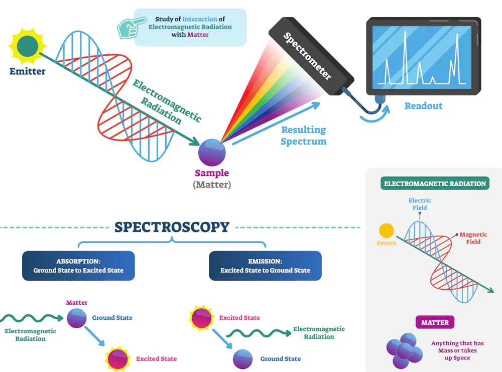
Just as fingerprinting uniquely identifies a person, scientists use spectroscopy to determine the chemical identity of microplastics. In spectroscopy, a substance either absorbs or scatters light, depending on how its molecules vibrate. The absorbed or scattered light creates a unique pattern called the spectrum, which is effectively the substance’s fingerprint.

A diagram showing how electromagnetic radiation interacting with a sample chemical generates a spectrum.
Spectroscopy can match a substance with its unique fingerprint.
VectorMine/iStock via Getty Images Plus

Just like a forensic analyst can match an unknown fingerprint against a fingerprint database to identify the person, researchers can match the spectrum of an unknown microplastic particle against a database of known spectra.

However, forensic analysts can get false matches in fingerprint matching. Similarly, spectral matching against a database isn’t foolproof. Many plastic polymers have similar structures, so two different polymers can have similar spectra. This overlap can lead to ambiguity in the identification process.

So, an identification method for polymers should provide a measure of uncertainty in its output. That way, the user can know how much to trust the polymer fingerprint match. Unfortunately, current methods don’t usually provide an uncertainty measure.

Data from microplastic analyses can inform health recommendations and policy decisions, so it’s important for the people making those calls to know how reliable the analysis is.

Conformal prediction

Machine learning is one tool researchers have started using for microplastic identification.

First, researchers collect a large dataset of spectra whose identities are known. Then, they use this dataset to train a machine learning algorithm that learns to predict a substance’s chemical identity from its spectrum.

Sophisticated algorithms whose inner workings can be opaque make these predictions, so the lack of an uncertainty measure becomes an even greater problem when machine learning is involved.

Our recent work addresses this issue by creating a tool with an uncertainty quantification for microplastic identification. We use a machine learning technique called conformal prediction.

Conformal prediction is like a wrapper around an existing, already trained machine learning algorithm that adds an uncertainty quantification. It does not require the user of the machine learning algorithm to have any detailed knowledge of the algorithm or its training data. The user just needs to be able to run the prediction algorithm on a new set of spectra.

To set up conformal prediction, researchers collect a calibration set containing spectra and their true identities. The calibration set is often much smaller than the training data required for training machine learning algorithms. Usually just a few hundred spectra are enough for calibration.

Then, conformal prediction analyzes the discrepancies between the predictions and correct answers in the calibration set. Using this analysis, it adds other plausible identities to the algorithm’s single output on a particular particle’s spectrum. Instead of outputting one, possibly incorrect, prediction like “this particle is polyethylene,” it now outputs a set of predictions – for example, “this particle could be polyethylene or polypropylene.”

The prediction sets contain the true identity with a level of confidence that users can set themselves – say, 90%. Users can then rerun the conformal prediction with a higher confidence – say, 95%. But the higher the confidence level, the more polymer predictions given by the model in the output.

It might seem that a method that outputs a set rather than a single identity isn’t as useful. But the size of the set serves as a way to assess uncertainty – a small set indicates less uncertainty.

On the other hand, if the algorithm predicts that the sample could be many different polymers, there’s substantial uncertainty. In this case, you could bring in a human expert to examine the polymer closely.

Testing the tool

To run our conformal prediction, my team used libraries of microplastic spectra from the Rochman Lab at the University of Toronto as the calibration set.

Once calibrated, we collected samples from a parking lot in Brighton, Michigan, obtained their spectra, and ran them through the algorithm. We also asked an expert to manually label the spectra with the correct polymer identities. We found that conformal prediction did produce sets that included the label the human expert gave it.

Two very similar looking line graphs, each with a large peaks and a few smaller peaks.
Some spectra, such as polyethylene on the left and polypropylene on the right, look very similar and can easily be confused. That’s why having an uncertainty measure can be helpful.
Ambuj Tewari

Microplastics are an emerging concern worldwide. Some places such as California have begun to gather evidence for future legislation to help curb microplastic pollution.

Evidence-based science can help researchers and policymakers fully understand the extent of microplastic pollution and the threats it poses to human welfare. Building and openly sharing machine learning-based tools is one way to help make that happen.The Conversation

Ambuj Tewari, Professor of Statistics, University of Michigan

This article is republished from The Conversation under a Creative Commons license. Read the original article.

Read More

The post What’s that microplastic? Advances in machine learning are making identifying plastics in the environment more reliable appeared first on theconversation.com

The Conversation

What causes the powerful winds that fuel dust storms, wildfires and blizzards? A weather scientist explains

Published

on

theconversation.com – Chris Nowotarski, Associate Professor of Atmospheric Science, Texas A&M University – 2025-03-20 07:49:00

When huge dust storms like this one in the Phoenix suburbs in 2022 hit, it’s easy to see the power of the wind.
Christopher Harris/iStock Images via Getty Plus

Chris Nowotarski, Texas A&M University

Windstorms can seem like they come out of nowhere, hitting with a sudden blast. They might be hundreds of miles long, stretching over several states, or just in your neighborhood.

But they all have one thing in common: a change in air pressure.

Just like air rushing out of your car tire when the valve is open, air in the atmosphere is forced from areas of high pressure to areas of low pressure.

The stronger the difference in pressure, the stronger the winds that will ultimately result.

A weather map with a line between high and low pressure stretching across the U.S.
On this forecast for March 18, 2025, from the National Oceanic and Atmospheric Administration, ‘L’ represents low-pressure systems. The shaded area over New Mexico and west Texas represents strong winds and low humidity that combine to raise the risk of wildfires.
NOAA Weather Prediction Center

Other forces related to the Earth’s rotation, friction and gravity can also alter the speed and direction of winds. But it all starts with this change in pressure over a distance – what meteorologists like me call a pressure gradient.

So how do we get pressure gradients?

Strong pressure gradients ultimately owe their existence to the simple fact that the Earth is round and rotates.

Because the Earth is round, the sun is more directly overhead during the day at the equator than at the poles. This means more energy reaches the surface of the Earth near the equator. And that causes the lower part of the atmosphere, where weather occurs, to be both warmer and have higher pressure on average than the poles.

Nature doesn’t like imbalances. As a result of this temperature difference, strong winds develop at high altitudes over midlatitude locations, like the continental U.S. This is the jet stream, and even though it’s several miles up in the atmosphere, it has a big impact on the winds we feel at the surface.

Wind speed and direction in the upper atmosphere on March 14, 2025, show waves in the jet stream. Downstream of a trough in this wave, winds diverge and low pressure can form near the surface.
NCAR

Because Earth rotates, these upper-altitude winds blow from west to east. Waves in the jet stream – a consequence of Earth’s rotation and variations in the surface land, terrain and oceans – can cause air to diverge, or spread out, at certain points. As the air spreads out, the number of air molecules in a column decreases, ultimately reducing the air pressure at Earth’s surface.

The pressure can drop quite dramatically over a few days or even just a few hours, leading to the birth of a low-pressure system – what meteorologists call an extratropical cyclone.

The opposite chain of events, with air converging at other locations, can form high pressure at the surface.

In between these low-pressure and high-pressure systems is a strong change in pressure over a distance – a pressure gradient. And that pressure gradient leads to strong winds. Earth’s rotation causes these winds to spiral around areas of high and low pressure. These highs and lows are like large circular mixers, with air blowing clockwise around high pressure and counterclockwise around low pressure. This flow pattern blows warm air northward toward the poles east of lows and cool air southward toward the equator west of lows.

A maps shows pressure changes don't follow a straight line.
A map illustrates lines of surface pressure, called isobars, with areas of high and low pressure marked for March 14, 2025. Winds are strongest when isobars are packed most closely together.
Plymouth State University, CC BY-NC-SA

As the waves in the jet stream migrate from west to east, so do the surface lows and highs, and with them, the corridors of strong winds.

That’s what the U.S. experienced when a strong extratropical cyclone caused winds stretching thousands of miles that whipped up dust storms and spread wildfires, and even caused tornadoes and blizzards in the central and southern U.S. in March 2025.

Whipping up dust storms and spreading fires

The jet stream over the U.S. is strongest and often the most “wavy” in the springtime, when the south-to-north difference in temperature is often the strongest.

Winds associated with large-scale pressure systems can become quite strong in areas where there is limited friction at the ground, like the flat, less forested terrain of the Great Plains. One of the biggest risks is dust storms in arid regions of west Texas or eastern New Mexico, exacerbated by drought in these areas.

Downtown is barely visible through a haze of dust.
A dust storm hit Albuquerque, N.M., on March 18, 2025. Another dust storm a few dats earlier in Kansas caused a deadly pileup involving dozens of vehices on I-70.
AP Photo/Roberto E. Rosales

When the ground and vegetation are dry and the air has low relative humidity, high winds can also spread wildfires out of control.

Even more intense winds can occur when the pressure gradient interacts with terrain. Winds can sometimes rush faster downslope, as happens in the Rockies or with the Santa Ana winds that fueled devastating wildfires in the Los Angeles area in January.

Violent tornadoes and storms

Of course, winds can become even stronger and more violent on local scales associated with thunderstorms.

When thunderstorms form, hail and precipitation in them can cause the air to rapidly fall in a downdraft, causing very high pressure under these storms. That pressure forces the air to spread out horizontally when it reaches the ground. Meteorologists call these straight line winds, and the process that forms them is a downburst. Large thunderstorms or chains of them moving across a region can cause large swaths of strong wind over 60 mph, called a derecho.

Finally, some of nature’s strongest winds occur inside tornadoes. They form when the winds surrounding a thunderstorm change speed and direction with height. This can cause part of the storm to rotate, setting off a chain of events that may lead to a tornado and winds as strong as 300 mph in the most violent tornadoes.

YouTube video
How a tornado forms. Source: NOAA.

Tornado winds are also associated with an intense pressure gradient. The pressure inside the center of a tornado is often very low and varies considerably over a very small distance.

It’s no coincidence that localized violent winds from thunderstorm downbursts and tornadoes often occur amid large-scale windstorms. Extratropical cyclones often draw warm, moist air northward on strong winds from the south, which is a key ingredient for thunderstorms. Storms also become more severe and may produce tornadoes when the jet stream is in close proximity to these low-pressure centers. In the winter and early spring, cold air funneling south on the northwest side of strong extratropical cyclones can even lead to blizzards.

So, the same wave in the jet stream can lead to strong winds, blowing dust and fire danger in one region, while simultaneously triggering a tornado outbreak and a blizzard in other regions.The Conversation

Chris Nowotarski, Associate Professor of Atmospheric Science, Texas A&M University

This article is republished from The Conversation under a Creative Commons license. Read the original article.

Read More

The post What causes the powerful winds that fuel dust storms, wildfires and blizzards? A weather scientist explains appeared first on theconversation.com

Continue Reading

The Conversation

5 years on, true counts of COVID-19 deaths remain elusive − and research is hobbled by lack of data

Published

on

theconversation.com – Dylan Thomas Doyle, Ph.D. Candidate in Information Science, University of Colorado Boulder – 2025-03-20 07:47:00

National COVID-19 memorial wall for the five-year anniversary on March 11, 2025, in London, England.
Andrew Aitchison/In Pictures via Getty Images

Dylan Thomas Doyle, University of Colorado Boulder

In the early days of the COVID-19 pandemic, researchers struggled to grasp the rate of the virus’s spread and the number of related deaths. While hospitals tracked cases and deaths within their walls, the broader picture of mortality across communities remained frustratingly incomplete.

Policymakers and researchers quickly discovered a troubling pattern: Many deaths linked to the virus were never officially counted. A study analyzing data from over 3,000 U.S. counties between March 2020 and August 2022 found nearly 163,000 excess deaths from natural causes that were missing from official mortality records.

Excess deaths, meaning those that exceed the number expected based on historical trends, serve as a key indicator of underreported deaths during health crises. Many of these uncounted deaths were later tied to COVID-19 through reviews of medical records, death certificates and statistical modeling.

In addition, lack of real-time tracking for medical interventions during those early days slowed vaccine development by delaying insights into which treatments worked and how people were responding to newly circulating variants.

Five years since the beginning of COVID-19, new epidemics such as bird flu are emerging worldwide, and researchers are still finding it difficult to access the data about people’s deaths that they need to develop lifesaving interventions.

How can the U.S. mortality data system improve? I’m a technology infrastructure researcher, and my team and I design policy and technical systems to reduce inefficiency in health care and government organizations. By analyzing the flow of mortality data in the U.S., we found several areas of the system that could use updating.

Critical need for real-time data

A death record includes key details beyond just the fact of death, such as the cause, contributing conditions, demographics, place of death and sometimes medical history. This information is crucial for researchers to be able to analyze trends, identify disparities and drive medical advances.

Approximately 2.8 million death records are added to the U.S. mortality data system each year. But in 2022 – the most recent official count available – when the world was still in the throes of the pandemic, 3,279,857 deaths were recorded in the federal system. Still, this figure is widely considered to be a major undercount of true excess deaths from COVID-19.

In addition, real-time tracking of COVID-19 mortality data was severely lacking. This process involves the continuous collection, analysis and reporting of deaths from hospitals, health agencies and government databases by integrating electronic health records, lab reports and public health surveillance systems. Ideally, it provides up-to-date insights for decision-making, but during the COVID-19 pandemic, these tracking systems lagged and failed to generate comprehensive data.

Two health care workers in full PPE attending to a patient lying on hospital bed
Getting real-time COVID-19 data from hospitals and other agencies into the hands of researchers proved difficult.
Gerald Herbert/AP Photo

Without comprehensive data on prior COVID-19 infections, antibody responses and adverse events, researchers faced challenges designing clinical trials to predict how long immunity would last and optimize booster schedules.

Such data is essential in vaccine development because it helps identify who is most at risk, which variants and treatments affect survival rates, and how vaccines should be designed and distributed. And as part of the broader U.S. vital records system, mortality data is essential for medical research, including evaluating public health programs, identifying health disparities and monitoring disease.

At the heart of the problem is the inefficiency of government policy, particularly outdated public health reporting systems and slow data modernization efforts that hinder timely decision-making. These long-standing policies, such as reliance on paper-based death certificates and disjointed state-level reporting, have failed to keep pace with real-time data needs during crises such as COVID-19.

These policy shortcomings lead to delays in reporting and lack of coordination between hospital organizations, state government vital records offices and federal government agencies in collecting, standardizing and sharing death records.

History of US mortality data

The U.S. mortality data system has been cobbled together through a disparate patchwork of state and local governments, federal agencies and public health organizations over the course of more than a century and a half. It has been shaped by advances in public health, medical record-keeping and technology. From its inception to the present day, the mortality data system has been plagued by inconsistencies, inefficiencies and tensions between medical professionals, state governments and the federal government.

The first national efforts to track information about deaths began in the 1850s when the U.S. Census Bureau started collecting mortality data as part of the decennial census. However, these early efforts were inconsistent, as death registration was largely voluntary and varied widely across states.

In the early 20th century, the establishment of the National Vital Statistics System brought greater standardization to mortality data. For example, the system required all U.S. states and territories to standardize their death certificate format. It also consolidated mortality data at the federal level, whereas mortality data was previously stored at the state level.

However, state and federal reporting remained fragmented. For example, states had no unifom timeline for submitting mortality data, resulting in some states taking months or even years to finalize and release death records. Local or state-level paperwork processing practices also remained varied and at times contradictory.

Close-up of blank form titled CERTIFICATE OF DEATH
Death record processing varies by state.
eric1513/iStock via Getty Images Plus

To begin to close gaps in reporting timelines to aid medical researchers, in 1981 the National Center for Health Statistics – a division of the Centers for Disease Control and Prevention – introduced the National Death Index. This is a centralized database of death records collected from state vital statistics offices, making it easier to access death data for health and medical research. The system was originally paper-based, with the aim of allowing researchers to track the deaths of study participants without navigating complex bureaucracies.

As time has passed, the National Death Index and state databases have become increasingly digital. The rise of electronic death registration systems in recent decades has improved processing speed when it comes to researchers accessing mortality data from the National Death Index. However, while the index has solved some issues related to gaps between state and federal data, other issues, such as high fees and inconsistency in state reporting times, still plague it.

Accessing the data that matters most

With the Trump administration’s increasing removal of CDC public health datasets, it is unclear whether policy reform for mortality data will be addressed anytime soon.

Experts fear that the removal of CDC datasets has now set precedent for the Trump administration to cross further lines in its attempts to influence the research and data published by the CDC. The longer-term impact of the current administration’s public health policy on mortality data and disease response are not yet clear.

What is clear is that five years since COVID-19, the U.S. mortality tracking system remains unequipped to meet emerging public health crises. Without addressing these challenges, the U.S. may not be able to respond quickly enough to public health crises threatening American lives.The Conversation

Dylan Thomas Doyle, Ph.D. Candidate in Information Science, University of Colorado Boulder

This article is republished from The Conversation under a Creative Commons license. Read the original article.

Read More

The post 5 years on, true counts of COVID-19 deaths remain elusive − and research is hobbled by lack of data appeared first on theconversation.com

Continue Reading

The Conversation

Atlantic sturgeon were fished almost to extinction − ancient DNA reveals how Chesapeake Bay population changed over centuries

Published

on

theconversation.com – Natalia Przelomska, Research Associate in Archaeogenomics, National Museum of Natural History, Smithsonian Institution – 2025-03-20 07:47:00

Sturgeon can be several hundred pounds each.
cezars/E+ via Getty Images

Natalia Przelomska, Smithsonian Institution and Logan Kistler, Smithsonian Institution

Sturgeons are one of the oldest groups of fishes. Sporting an armor of five rows of bony, modified scales called dermal scutes and a sharklike tail fin, this group of several-hundred-pound beasts has survived for approximately 160 million years. Because their physical appearance has changed very little over time, supported by a slow rate of evolution, sturgeon have been called living fossils.

Despite their survival through several geological time periods, many present-day sturgeon species are at threat of extinction, with 17 of 27 species listed as “critically endangered.”

Conservation practitioners such as the Virginia Commonwealth University monitoring team are working hard to support recovery of Atlantic sturgeon in the Chesapeake Bay area. But it’s not clear what baseline population level people should strive toward restoring. How do today’s sturgeon populations compare with those of the past?

Three people carefully lower a large fish over the side of a boat toward the water
VCU monitoring team releases an adult Atlantic sturgeon back into the estuary.
Matt Balazik

We are a molecular anthropologist and a biodiversity scientist who focus on species that people rely on for subsistence. We study the evolution, population health and resilience of these species over time to better understand humans’ interaction with their environments and the sustainability of food systems.

For our recent sturgeon project, we joined forces with fisheries conservation biologist Matt Balazik, who conducts on-the-ground monitoring of Atlantic sturgeon, and Torben Rick, a specialist in North American coastal zooarchaeology. Together, we wanted to look into the past and see how much sturgeon populations have changed, focusing on the James River in Virginia. A more nuanced understanding of the past could help conservationists better plan for the future.

Sturgeon loomed large for millennia

In North America, sturgeon have played important subsistence and cultural roles in Native communities, which marked the seasons by the fishes’ behavioral patterns. Large summertime aggregations of lake sturgeon (Acipenser fulvescens) in the Great Lakes area inspired one folk name for the August full moon – the sturgeon moon. Woodland Era pottery remnants at archaeological sites from as long as 2,000 years ago show that the fall and springtime runs of Atlantic sturgeon (Acipenser oxyrinchus) upstream were celebrated with feasting.

triangular-shaped bone with round cavities
Archaeologists uncover bony scutes – modified scales that resemble armor for the living fish – in places where people relied on sturgeon for subsistence.
Logan Kistler and Natalia Przelomska

Archaeological finds of sturgeon remains support that early colonial settlers in North America, notably those who established Jamestown in the Chesapeake Bay area in 1607, also prized these fish. When Captain John Smith was leading Jamestown, he wrote “there was more sturgeon here than could be devoured by dog or man.” The fish may have helped the survival of this fortress-colony that was both stricken with drought and fostering turbulent relationships with the Native inhabitants.

This abundance is in stark contrast to today, when sightings of migrating fish are sparse. Exploitation during the past 300 years was the key driver of Atlantic sturgeon decline. Demand for caviar drove the relentless fishing pressure throughout the 19th century. The Chesapeake was the second-most exploited sturgeon fishery on the Eastern Seaboard up until the early 20th century, when the fish became scarce.

Man pulls large fish over side of boat
Conservation biologists capture the massive fish for monitoring purposes, which includes clipping a tiny part of the fin for DNA analysis.
Matt Balazik

At that point, local protection regulations were established, but only in 1998 was a moratorium on harvesting these fish declared. Meanwhile, abundance of Atlantic sturgeon remained very low, which can be explained in part by their lifespan. Short-lived fish such as herring and shad can recover population numbers much faster than Atlantic sturgeon, which live for up to 60 years and take a long time to reach reproductive age – up to around 12 years for males and as many as 28 years for females.

To help manage and restore an endangered species, conservation biologists tend to split the population into groups based on ranges. The Chesapeake Bay is one of five “distinct population segments” the U.S. Endangered Species Act listing in 2012 created for Atlantic sturgeon.

Since then, conservationists have pioneered genetic studies on Atlantic sturgeon, demonstrating through the power of DNA that natal river – where an individual fish is born – and season of spawning are both important for distinguishing subpopulations within each regional group. Scientists have also described genetic diversity in Atlantic sturgeon; more genetic variety suggests they have more capacity to adapt when facing new, potentially challenging conditions.

map highlighting Maycock's Point, Hatch Site, Jamestown and Williamsburg on the James River
The study focused on Atlantic sturgeon from the Chesapeake Bay region, past and present. The four archaeological sites included are highlighted.
Przelomska NAS et al., Proc. R. Soc. B 291: 20241145, CC BY

Sturgeon DNA, then and now

Archaeological remains are a direct source of data on genetic diversity in the past. We can analyze the genetic makeup of sturgeons that lived hundreds of years ago, before intense overfishing depleted their numbers. Then we can compare that baseline with today’s genetic diversity.

The James River was a great case study for testing out this approach, which we call an archaeogenomics time series. Having obtained information on the archaeology of the Chesapeake region from our collaborator Leslie Reeder-Myers, we sampled remains of sturgeon – their scutes and spines – at a precolonial-era site where people lived from about 200 C.E. to about 900 C.E. We also sampled from important colonial sites Jamestown (1607-1610) and Williamsburg (1720-1775). And we complemented that data from the past with tiny clips from the fins of present-day, live fish that Balazik and his team sampled during monitoring surveys.

scattering of small bone shards spilling out of ziplock bag, with a purple-gloved hand
Scientists separate Atlantic sturgeon scute fragments from larger collections of zooarchaeological remains, to then work on the scutes in a lab dedicated to studying ancient DNA.
Torben Rick and Natalia Przelomska

DNA tends to get physically broken up and biochemically damaged with age. So we relied on special protocols in a lab dedicated to studying ancient DNA to minimize the risk of contamination and enhance our chances of successfully collecting genetic material from these sturgeon.

Atlantic sturgeon have 122 chromosomes of nuclear DNA – over five times as many as people do. We focused on a few genetic regions, just enough to get an idea of the James River population groupings and how genetically distinct they are from one another.

We were not surprised to see that fall-spawning and spring-spawning groups were genetically distinct. What stood out, though, was how starkly different they were, which is something that can happen when a population’s numbers drop to near-extinction levels.

We also looked at the fishes’ mitochondrial DNA, a compact molecule that is easier to obtain ancient DNA from compared with the nuclear chromosomes. With our collaborator Audrey Lin, we used the mitochondrial DNA to confirm our hypothesis that the fish from archaeological sites were more genetically diverse than present-day Atlantic sturgeon.

Strikingly, we discovered that mitochondrial DNA did not always group the fish by season or even by their natal river. This was unexpected, because Atlantic sturgeon tend to return to their natal rivers for breeding. Our interpretation of this genetic finding is that over very long timescales – many thousands of years – changes in the global climate and in local ecosystems would have driven a given sturgeon population to migrate into a new river system, and possibly at a later stage back to its original one. This notion is supported by other recent documentation of fish occasionally migrating over long distances and mixing with new groups.

Our study used archaeology, history and ecology together to describe the decline of Atlantic sturgeon. Based on the diminished genetic diversity we measured, we estimate that the Atlantic sturgeon populations we studied are about a fifth of what they were before colonial settlement. Less genetic variability means these smaller populations have less potential to adapt to changing conditions. Our findings will help conservationists plan into the future for the continued recovery of these living fossils.The Conversation

Natalia Przelomska, Research Associate in Archaeogenomics, National Museum of Natural History, Smithsonian Institution and Logan Kistler, Curator of Archaeobotany and Archaeogenomics, National Museum of Natural History, Smithsonian Institution

This article is republished from The Conversation under a Creative Commons license. Read the original article.

Read More

The post Atlantic sturgeon were fished almost to extinction − ancient DNA reveals how Chesapeake Bay population changed over centuries appeared first on theconversation.com

Continue Reading

Trending